Extract forceconstants

Short description

The main algorithm of the TDEP method. Starting with a symmetry analysis, this code finds the irreducible representation of interatomic forceconstants and extracts them from position and force data.

Command line options:

Optional switches:

--secondorder_cutoff value, -rc2 value
default value 5.0
Cutoff for the second order force constants
--thirdorder_cutoff value, -rc3 value
default value -1 mutually exclude "--thirdorder_njump"
Cutoff for the third order force constants
--fourthorder_cutoff value, -rc4 value
default value -1 mutually exclude "--fourthorder_njump"
Cutoff for the fourth order force constants
--polar
default value .false.
Add dipole-dipole corrections for polar materials.
--stride value, -s value
default value 1
Use every N configuration instead of all. Useful for long MD simulations with linearly dependent configurations.
--firstorder
default value .false.
Include the first order force constants. These can be used to find the finite temperature equilibrium structure.
--temperature value
default value -1
Temperature for self-consistent solver.
--norotational
default value .false.
Turn off imposing rotational invariance. Needed for 2D systems.
--nohuang
default value .false.
Turn off imposing Huang invariances. Useful for 2D systems.
--nohermitian
default value .false.
--help, -h
Print this help message
--version, -v
Print version

Examples

extract_forceconstants -rc2 5.1

extract_forceconstants -rc2 4.5 -rc3 3.21

Longer summary

Calculations of the interatomic force constants are the most important part of any lattice dynamics calculation as they are used to calculate many micro and macroscopic properties of the system, e.g. phonon, thermodynamic, and transport properties, etc. This codes takes sets of displacements and forces, and uses these to fit the coefficients in an effective lattice dynamical Hamiltonian. This is by no means a new idea.⁵ The main advantage of the TDEP method is in the implementation: it is numerically robust, well tested and general.

What is a force constant model

Interatomic force constants are a central quantity in the TDEP model. The idea is to express the Born-Oppenheimer potential energy surface as a low-order polynomial around some configuration of interest. A quick recap of lattice dynamical theory:⁶ a displacement \(\mathbf{u}\) of an atom \(i\) from its ideal lattice position changes the potential energy of the lattice. Temperature disorders the lattice, causing all atoms to be displaced from their equilibrium positions; this effect can be modeled as a Taylor expansion of the potential energy contribution of the instantaneous positions of the atoms in the system, i.e. \(U=U(\{ \mathbf{r} \})\). It is convenient to define the atomic positions as displacements \(\mathbf{u}\) from their equilibrium positions \(\mathbf{R}_i+\boldsymbol{\tau}_i\).

\[ \begin{equation} \textbf{r}_i=\mathbf{R}_i+\boldsymbol{\tau}_i+\mathbf{u}_i. \end{equation} \]

\(\mathbf{R}_i\) is a lattice vector and \(\boldsymbol{\tau}_i\) is the position in the unit cell. We can then expand the potential energy in terms of displacements as:

\[ \begin{equation} \begin{split} U(\{\textbf{u}\})=& U_0+ \sum_{i}\sum_\alpha \Phi^\alpha_{i} u^\alpha_{i} + \frac{1}{2!} \sum_{ij} \sum_{\alpha\beta} \Phi^{\alpha\beta}_{ij} u^\alpha_{i} u^\beta_{j} + \\ + & \frac{1}{3!} \sum_{ijk} \sum_{\alpha\beta\gamma} \Phi^{\alpha\beta\gamma}_{ijk} u^\alpha_{i} u^\beta_{j} u^\gamma_{k}+ \frac{1}{4!} \sum_{ijkl} \sum_{\alpha\beta\gamma\delta} \Phi^{\alpha\beta\gamma\delta}_{ijkl} u^\alpha_{i} u^\beta_{j} u^\gamma_{k} u^\delta_{l} + \ldots \end{split} \end{equation} \]

Here, \(\alpha\beta\gamma\delta\) are Cartesian indices and \(U_0\) is the potential energy of the static lattice. The coefficients of the Taylor expansion are the derivatives of the potential energy with respect to displacement and are called the Born-von Kàrmàn force constants, which can be expressed as tensors of increasing rank:

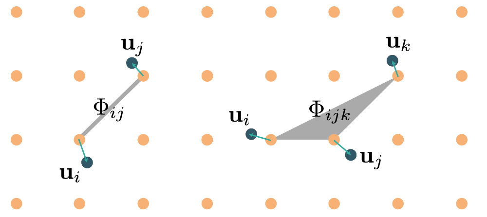
\[ \begin{align} \Phi^\alpha_i & = \left. \frac{\partial U}{\partial u_i^\alpha} \right|_{u=0} = 0 \\ \Phi^{\alpha\beta}_{ij} & = \left. \frac{\partial^2 U}{\partial u_i^\alpha \partial u_j^\beta} \right|_{u=0} \\ \Phi^{\alpha\beta\gamma}_{ijk} & = \left. \frac{\partial^3 U}{\partial u_i^\alpha \partial u_j^\beta \partial u_k^\gamma} \right|_{u=0} \\ \Phi^{\alpha\beta\gamma\delta}_{ijkl} & = \left. \frac{\partial^4 U}{\partial u_i^\alpha \partial u_j^\beta \partial u_k^\gamma \partial u_l^\delta} \right|_{u=0} \end{align} \]

By increasing rank, the force constants of rank \(n\) represent \(n\)-body interactions, as illustrated in the diagram below:

What differs in the TDEP method and the textbook definitions is that we do not consider the interaction tensors as a Taylor expansion, instead they are free parameters designed to best describe the system at elevated temperature. This is done via a fitting procedure that will be explained below, and prefaced with a short formal motivation. The main advantage of a force constant model over the raw Born-Oppenheimer potential energy surface is that once it is established a host of quantities can be determined -- detailed in all the other sections of this manual.

Motivation for least squares fitting procedure

Let's take a few steps back. Suppose we have the correct Hamiltonian \(H_1\) then we can evaluate, but it involves a substantial computational effort. It is then beneficial to create a model Hamiltonian \(H_0\) that is as close as possible to \(H_1\), but is several orders of magnitude cheaper to deal with computationally.

For now, I will call \(H_1\) the true Hamiltonian, and \(H_0\) the reference Hamiltonian. I assume we have the means to numerically evaluate \(H_1\), but doing so is expensive. In this context, any numerical evaluation of \(H_0\) is considered to have negligible cost. The task is to evaluate the best criteria to use for determining \(H_0\), using information from \(H_1\), such that \(H_0\) can be used to evaluate physical properties of the system in question. This idea has been around since forever, and this secontion is a short recap of all the historical efforts to do so.

Work

Not the kind you are supposed to be doing, but the kind you were supposed to pay attention to in class. I have already defined our two Hamiltonians, \(H_0\) and \(H_1\). We start by defining an alchemical coupling path between the two Hamiltonians:

\[\label{eq:kirkwood} H(\lambda) = (1-\lambda) H_0 + \lambda H_1 \]

as a quantity to work with. The parameter \(0<\lambda<1\) allows us to alchemically switch between the Hamiltonians, or viewed differently, apply work to/measure work done by the systemfrom \(H_1\) to \(H_0\) and vice versa. Per some textbook we know that

\[ \begin{equation}\label{eq:workandstuff} \Delta F \le W \end{equation} \]

the free energy difference is smaller than the work done by the system. Think this is where the term free energy comes from, the energy free to do work. The equality holds in the quasistatic limit, where the system is kept in equilibrium the whole time. This leads is to one way to determine the free energy, Kirkwood coupling:

\[\label{eq:termoint} F_1-F_0 = \int_0^1 \frac{\partial F(\lambda)}{\partial \lambda} d{\lambda} = \int_0^1 \left\langle H_1-H_0 \right\rangle_{\lambda} d{\lambda} \]

This is the same as \(\ref{eq:workandstuff}\). Here I introduced a new notation:

\[ \left\langle X \right\rangle_y = \int X e^{ -\beta H_y} d{\vec{p}}d{\vec{r}} \]

That is, the angled brackets means configuration average with respect to Hamiltonian \(y\). Works quantum mechical as well, just replace the integral with \(\textrm{ln} \textrm{tr}\). Good homework exercise to show (just write down the classical partition function for \(H(\lambda)\) and take the derivative w.r.t \(\lambda\), and it falls out by itself, remembering that \(F=-k_B T \ln Z\)).

At this point we are not interested in performing the integration over \(\lambda\), although it certainly is practically possible if one wants to. Rather we will use this expression backwards, i.e. figure out a way to make \(H_1-H_0\) as small as possible, since then the difference in free energy should disappear. And we can do this in a rather neat way. Several ways actually, but they all lead to the same result.

Expand along alchemical path

First, we can expand \(F(\lambda)\) around \(\lambda=0\)

\[ \begin{equation} \begin{split} F(\lambda) = & F_0 + \left\langle H_1-H_0 \right\rangle_0\lambda + \\ & \beta \left( \left\langle(H_1-H_0)^2 \right\rangle_0-\left\langle H_1-H_0 \right\rangle^2_{0} \right)\lambda^2 + \sum_{n=3}^{\infty} \frac{1}{n!} C_0^n \lambda^n \end{split} \end{equation} \]

And integrate this from \(\lambda=0\) to \(\lambda=1\) and arrive at

\[ \begin{equation} \begin{split} F_1 = & F_0 + \left\langle H_1-H_0 \right\rangle_0 + \\ & \frac{\beta}{2} \left( \left\langle(H_1-H_0)^2 \right\rangle_0-\left\langle H_1-H_0 \right\rangle^2_{0} \right) + \sum_{n=3}^{\infty} C_0^n \end{split} \end{equation} \]

We can also expand around \(\lambda=1\), and arrive at

\[ \begin{equation} \begin{split} F_0 = & F_1 + \left\langle H_1-H_0 \right\rangle_1 + \\ & \frac{\beta}{2} \left( \left\langle(H_1-H_0)^2 \right\rangle_1-\left\langle H_1-H_0 \right\rangle^2_{1} \right) + \sum_{n=3}^{\infty} C_1^n \end{split} \end{equation} \]

Here the sum of \(C_0^n\) runs of all the cumulants of order 3 and higher, with measure \(H_0\) and \(H_1\), respectively. Alternatively, one could start from an alternative exact expression:

\[ F_A = F_B - k_B T \ln \left\langle \exp(-\beta(H_A-H_B)) \right\rangle \]

And do a cumulant expansion and arrive at exactly the same expressions. This is by no means a new idea,⁴²³ and by tracing references backwards I ended up at Thiele semiinvariants from 1800-something but could not find the actual papers. Suffice to say that is established.

Constraining the free energy

We then make use of the Gibbs-Bogoliubov inequality (unfairly named since that also seems to trace much further back in time) that states

\[ F_1 \le F_0 + \left\langle H_1-H_0 \right\rangle_0 \]

or

\[ F_0 \ge F_1 + \left\langle H_1-H_0 \right\rangle_1 \]

by simple relabelling of terms. If we now insert or expansion expressions into the inequalities we end up with

\[ 0 \le \frac{2}{\beta} \sum_{n=3}^{\infty} C_1^n \le \left\langle(H_1-H_0)^2 \right\rangle_0-\left\langle H_1-H_0 \right\rangle^2_{0} \]

and

\[ 0 \le \frac{2}{\beta} \sum_{n=3}^{\infty} C_1^n \le \left\langle(H_1-H_0)^2 \right\rangle_1-\left\langle H_1-H_0 \right\rangle^2_{1} \]

What this means is that the second term in the expansion is larger than the sum of all higher order terms. So, to minimize the difference in free energy between \(H_0\) and \(H_1\), we need to minimize the variance of the energy, either samples with the proper dynamics \(\langle\rangle_1\) or via approximate dynamics \(\langle\rangle_0\).

Conclusion

What I sketched above is that the Gibbs-Bogoliubov inequality can be recast into the problem of minimizing variance between a model Hamiltonian and the exact Hamiltonian, and that you are free to choose which statistical measure to use -- the result will be variational with respect to the free energy. This serves as the formal motivation behind TDEP. One option is to run ab inito (path integral) molecular dynamics to sample the potential energy surface, that would correspond to using measure \(\langle\rangle_1\). The other option is to use self-consistent stochastic sampling, this corresponds to \(\langle\rangle_1\) and is equivalent to self-consistent phonons.

The main benefit of the above is that instead of minimizing an expression that involves three free energy, we minimize an expression that only involves the internal energy which is a lot easier. And since it is a variance we are to minimize a least squares solution is the natural choice, the least squares solution is the minimum variance solution. The variance is the square you minimize.

Admittedly, this is a rather rough sketch of a motivation, a far more rigorous treatment is given by Alois, Jose and Matt, but the conclusions are the same.

Note

Fix reference to mode coupling paper as soon as it's published properly.

Practical procedure

Now that we have established that a least squares fit of a model Hamiltonian is in general a good idea we have to do it in practice. The first step is to simplify the problem using symmetry.

Force constant symmetries

Symmetry analysis allows us to greatly reduce the number of values needed to express the force constants and is therefore crucial for generalizing the TDEP to include higher order terms in the potential energy surface. The symmetries of the force constants are deduced from rotational and translational invariance of the system, in addition to the symmetries of the crystal itself. We start with the transposition symmetries, which is an invariance under the permutation of the indices:⁹⁸

\[ \begin{align} \Phi_{ij}^{\alpha\beta} & = \Phi_{ji}^{\beta\alpha} \\ \Phi_{ijk}^{\alpha\beta\gamma} & = \Phi_{jik}^{\beta\alpha\gamma} = \ldots \\ \Phi_{ijkl}^{\alpha\beta\gamma\delta} & = \Phi_{jikl}^{\alpha\beta\gamma\delta} = \ldots \end{align} \]

All lattices belong to one of the 230 lattice space groups. The force constants should be invariant under these symmetry operations. If two tensors are related by symmetry operation \(S\) their components are related as follows:

\[ \begin{align} \Phi_{ij}^{\alpha\beta} &= \sum_{\mu\nu}\Phi_{kl}^{\mu\nu} S^{\mu\alpha}S^{\nu\beta} \\ \Phi_{ijk}^{\alpha\beta\gamma} &= \sum_{\mu\nu\xi}\Phi_{mno}^{\mu\nu\xi} S^{\mu\alpha} S^{\nu\beta} S^{\xi\gamma}\\ \Phi_{ijkl}^{\alpha\beta\gamma\delta} &= \sum_{\mu\nu\xi\kappa}\Phi_{mnop}^{\mu\nu\xi\kappa} S^{\mu\alpha} S^{\nu\beta} S^{\xi\gamma} S^{\kappa\delta} \,.\\ \end{align} \]

where \(S^{\alpha\beta}\) is the proper or improper rotation matrix of the symmetry operation \(S\). Naturally, this will also enforce the periodic nature of the lattice. Force constants also obey the translational invariance (acoustic sum rules):

\[ \begin{align} \sum_j \mathbf{\Phi}_{ij} & =0 \quad \forall\, i \\ \sum_k \mathbf{\Phi}_{ijk} & =0 \quad \forall\, i,j \\ \sum_l \mathbf{\Phi}_{ijkl} & =0 \quad \forall\, i,j,k \end{align} \]

The rotational invariance gives

\[ \begin{align} \sum_i \Phi_i^\alpha r_i^\beta & = \sum_i \Phi_i^\beta r_i^\alpha \quad \forall \, \alpha,\beta \\ \sum_j \Phi_{ij}^{\alpha\beta} r_j^\gamma + \Phi_i^\beta \delta_{\alpha\gamma} & = \sum_j \Phi_{ij}^{\alpha\gamma} r_j^\beta + \Phi_i^\gamma \delta_{\alpha\beta} \quad \forall \, \alpha,\beta,\gamma \\ \sum_k \Phi_{ijk}^{\alpha\beta\gamma}r_k^\lambda + \Phi_{ij}^{\gamma\beta} \delta_{\alpha\lambda} + \Phi_{ij}^{\alpha\gamma} \delta_{\beta\lambda} &= \sum_k \Phi_{ijk}^{\alpha\beta\lambda}r_k^\gamma + \Phi_{ij}^{\lambda\beta} \delta_{\alpha\gamma} + \Phi_{ij}^{\alpha\lambda} \delta_{\beta\gamma} \quad \forall \, \alpha,\beta,\gamma,\lambda \\ \end{align} \]

And finally, the Huang invariances

\[ \begin{align} [\alpha\beta,\gamma\lambda] & = \sum_{ij} \Phi_{ij}^{\alpha\beta} r_{ij}^\gamma r_{ij}^\lambda \\ [\alpha\beta,\gamma\lambda] & = [\gamma\lambda,\alpha\beta] \end{align} \]

ensure that the second order forceconstants, when taken to the long-wavelength limit, result in the correct number of elastic constants. For low-symmetry crystals the Hermitian character of the dynamical matrix is enforced:¹⁴¹³

\[ \begin{equation} \sum_{j \ne i} \Phi^{\alpha\beta}_{ij} = \sum_{j \ne i} \Phi^{\beta\alpha}_{ij} \quad \forall\, i \end{equation} \]

All the symmetry relations above are naturally satisfied by the force constants produced by this code. In particular, the rotational, Huang and Hermitian invariances are rarely enforced in the literature, but are crucial for a correct behavior.

Note

A word of caution for low-dimensional systems: the Huang invariances do not apply there. Consider graphene, it is difficult to define an elastic constant that corresponds to compression along the z-axis in a meaningful way. The short term solution is to temporarily switch them off via the option --nohuang. The long term solution is to derive the proper invariances for a two-dimensional material, something I have not had the time to do.

Practical use of symmetries

The symmetry relations needs to be transformed to linear algebra to be of practical use. I will use the second order force constants as an example, but the procedure is general. First step is to flatten each \(3 \times 3\) tensor into a \(9 \times 1\) vector, and express each component of the tensor as a linear combination of some coefficients \(x\):

\[ \underbrace{\mathbf{\Phi}}_{9 \times 1} = \underbrace{\mathbf{C}}_{9 \times 1} \underbrace{\mathbf{x}}_{9 \times 1} \]

Suppose some (point) symmetry operators leave the tensor invariant, this can be expressed as

\[ \left(\sum_i \mathbf{S}_i \otimes \mathbf{S}_i - \mathbf{I}\right) \mathbf{\Phi} = 0 \]

There is also transposition symmetry, which can be expressed as a permutation matrix \(T\):

\[ \left(\mathbf{T} - \mathbf{I}\right) \mathbf{\Phi} = 0 \]

In total, this can be expressed as

\[ \mathbf{A} = \left(\mathbf{T} - \mathbf{I}\right) + \left(\sum_i \mathbf{S}_i \otimes \mathbf{S}_i - \mathbf{I}\right) \]

\[ \mathbf{A} \mathbf{C} \mathbf{x} = 0 \]

the problem is now reduced to finding \(\mathbf{C}\). We are not interested in the trivial solution \(\mathbf{C}=0\), instead we seek a matrix \(\mathbf{C}\) in the null space of \(\mathbf{A}\). We find that by constructing

\[ \mathbf{U}\mathbf{\Sigma}\mathbf{V} = A \]

\[ \mathbf{C} = \sum_{\Sigma_i = 0} \mathbf{U}^T \mathbf{V} \]

The rank of \(\mathbf{C}\) is the number of zero singular values of \(\mathbf{A}\), i.e. the number of irreducible variables \(\mathbf{x}\), resulting in

\[ \underbrace{\mathbf{\Phi}}_{9 \times 1} = \underbrace{\mathbf{C}}_{9 \times N_x} \underbrace{\mathbf{x}}_{N_x \times 1} \]

where \(N_x \le 9\).

Practical use in real systems

We use a procedure near identical to what is described above. The starting point is a set of displacements \(\vec{u}\) and forces \(\vec{f}\) from a set of \(N_c\) supercells sampled from a canonical ensemble at temperature \(T\). Although omitted in the notation, all interaction tensors depend on temperature as well as the volume (or more generally strain). The interatomic force constants are determined as follows: consider a supercell with \(N_a\) atoms and forces and displacements given by the \(3N_{a} \times 1\) vectors \(\vec{u}\) and \(\vec{f}\) (for clarity we will make note of the dimensions of the matrices in each step):

\[ \underbrace{\vec{f}}_{3N_a \times 1} = - \underbrace{\vec{\Phi}}_{3N_a \times 3 N_a} \underbrace{\vec{u}}_{3N_a \times 1} \]

we can arrange this on a form with flattened tensors as

\[ \underbrace{\vec{f}}_{3N_a \times 1} = - \underbrace{(\vec{I} \otimes \vec{u}^T)}_{3N_a \times (3N_a)^2} \underbrace{\vec{\Phi}_v}_{ (3N_a)^2 \times 1} \]

with the Kronecker product \(\otimes\). To express the forces from \(N_c\) supercells the matrices are stacked on top of each other:

\[ \underbrace{ \begin{pmatrix} \vec{f}_1 \\ \vdots \\ \vec{f}_{N_c} \end{pmatrix} }_{3N_a N_c \times 1} = - \underbrace{ \begin{pmatrix} \vec{I} \otimes \vec{u}_1^T \\ \vdots \\ \vec{I} \otimes \vec{u}_{N_c}^T \\ \end{pmatrix} }_{3N_aN_c \times (3N_a)^2} \underbrace{\vec{\Phi}_v}_{ (3N_a)^2 \times 1} \]

We then express the force constants via the irreducible components

\[ \underbrace{ \begin{pmatrix} \vec{f}_1 \\ \vdots \\ \vec{f}_{N_c} \end{pmatrix} }_{3N_a N_c \times 1} = - \underbrace{ \underbrace{ \begin{pmatrix} \vec{I} \otimes \vec{u}_1^T \\ \vdots \\ \vec{I} \otimes \vec{u}_{N_c}^T \\ \end{pmatrix} }_{3N_aN_c \times (3N_a)^2} \underbrace{ \vec{C}^{\Phi\textrm{II}} }_{(3N_a)^2 \times N_x} }_{=\vec{A}^{\Phi\textrm{II}}\,, 3N_a N_c \times N_x } \underbrace{\vec{x}^{\Phi\textrm{II}}}_{ N_x \times 1} \]

The set of symmetry relations and invariances determines \(\vec{C}\) and \(N_x\),~\cite{Leibfried1961,Maradudin1968,Born1998} and in general \(N_x \ll (3N_a)^2\) which considerably simplifies the problem of numerically determining \(\vec{\Phi}\). In practice, only the matrix \(\vec{A}\) is determined and stored. The nominally very large matrices that go into the construction of \(\vec{A}\) are quite sparse and construction presents negligible computational cost. The second order force constants imply matrices that could possibly be treated naively, but the generalization to higher order quickly becomes intractable with dense matrix storage. The third order force constants, for example, comes down to

\[ \underbrace{ \begin{pmatrix} \vec{f}_1 \\ \vdots \\ \vec{f}_{N_c} \end{pmatrix} }_{3N_a N_c \times 1} = - \underbrace{ \underbrace{ \begin{pmatrix} \vec{I} \otimes \vec{u}_1^T \otimes \vec{u}_1^T\\ \vdots \\ \vec{I} \otimes \vec{u}_{N_c}^T \otimes \vec{u}_{N_c}^T \\ \end{pmatrix} }_{3N_aN_c \times (3N_a)^3} \underbrace{ \vec{C}^{\Phi\textrm{III}} }_{(3N_a)^3 \times N_x} }_{=\vec{A}^{\Phi\textrm{III}}\,, 3N_a N_c \times N_x } \underbrace{\vec{x}^{\Phi\textrm{III}}}_{ N_x \times 1} \]

where the contracted matrix \(\vec{A}\) is many orders of magnitude smaller than the matrices it is built from.

The interatomic force constants are determined in succession:

\[ \begin{align} \label{eq:f2} \vec{A}^{\Phi\textrm{II}} \vec{x}^{\Phi\textrm{II}} & = \vec{f} % \\ % \label{eq:f3} \vec{A}^{\Phi\textrm{III}} \vec{x}^{\Phi\textrm{III}} & = \vec{f}- \vec{A}^{\Phi\textrm{II}} \vec{x}^{\Phi\textrm{II}} % \\ % \label{eq:f4} \vec{A}^{\Phi\textrm{IV}} \vec{x}^{\Phi\textrm{IV}} & = \vec{f} - \vec{A}^{\Phi\textrm{II}} \vec{x}^{\Phi\textrm{II}} - \vec{A}^{\Phi\textrm{III}} \vec{x}^{\Phi\textrm{III}} \end{align} \]

Where \(\vec{f}\) denotes the reference forces to be reproduced. Equations \(\ref{eq:f2}-\ref{eq:f4}\) are overdetermined and solved as a least squares problem. This ensures that the baseline harmonic part becomes as large as possible, and that the higher order terms become smaller and smaller. Some of the symmetry constraints are cumbersome to implement as linear operators, they are instead implemented as linear constraints. So for a low symmetry crystal the least squares problem is stated as

\[ \vec{A}^{\Phi\textrm{II}} \vec{x}^{\Phi\textrm{II}} = \vec{f} \quad \textrm{subject to} \quad \vec{B}\vec{x}^{\Phi\textrm{II}}=0 \]

On dynamical stability and stochastic sampling

Note

add link to stochastic sampling tutorial once it is prepared

As we established above we can either sample the potential energy surface via some variant of molecular dynamics/Monte Carlo simulations per the true Hamiltonian, or sample using the force constant model. Sampling with the force constant model collapses in case any eigenvalue of the dynamical matrix is negative - in that case no free energy is defined. One generally states self-consistent phonon theory as minimization of \(F_0 + \left\langle H_1 -H_0 \right\rangle_0\) with respect to the parameters in the model Hamiltonian. This is a slight simplification, since the symmetry constraints from the space group imply a reduced search space, some symmetry constraints imply additional equality constraints and on top of that we have the requirement of positive semi-definite eigenvalues.

Let's start from the naive least squares problem:

\[ \min_{\phi} \left\| F - U \Phi \right\|^2 \]

We use the same flattening technique as previously and can rewrite the least squares problem (by expanding the square) as

\[ \min_{\phi} \vec{\Phi_v}^T \left[\tilde{\vec{U}}^T\otimes\tilde{\vec{U}}\right] \vec{\Phi_v} - \vec{\Phi_v}^T \left[\vec{I}\otimes\tilde{\vec{U}}\right]^T \vec{F}_v \,. \]

The next step is to again express the force constants in terms of their irreducible components, and remember that we have some linear constraints:

\[ \begin{align} \vec{x} & = \min_{\vec{x}}\, \vec{x}^T \vec{D} \vec{x} - \vec{x}^T \vec{d} \quad \textrm{s.t.} \quad \vec{B}\vec{x}=0 \\ \vec{D} & = \vec{C}^T \left[\tilde{\vec{U}}^T\otimes\tilde{\vec{U}}\right] \vec{C} = \vec{A^T}\vec{A} \\ \vec{d} & = \vec{C}^T \left[\vec{I}\otimes\tilde{\vec{U}}\right]^T \vec{F}_v = \vec{A}^T \vec{F} \end{align} \]

The main difficulty lies in the constraint that the dynamical matrix needs to be positive semi-definite. This constraint can be states as

\[ \vec{s}^T \Phi \vec{s} > 0 \]

for any vector \(\vec{s}\), i.e. there is no combination of displacements that lower the energy below the baseline. In our flattened and irreducible form this becomes

\[ \vec{s} \otimes \vec{s} \vec{C} \vec{x} > 0 \]

Luckily, this is a solved problem.⁷ The algorithm progresses as follows: first we solve

\[ \vec{x} = \min_{\vec{x}}\, \vec{x}^T \vec{D} \vec{x} - \vec{x}^T \vec{d} \quad \textrm{s.t.} \quad \vec{B}\vec{x}=0 \, \]

and construct \(\Phi\), and examine the eigenvalues. If all eigenvalues are positive, we are done. If not, all the eigenvectors corresponding to negative eigenvalues are added as inequality constraints:

\[ \vec{E} = \left( \epsilon_1 \otimes \epsilon_1 \cdots \epsilon_N \otimes \epsilon_N \right)\vec{C} \]

and we get a new quadratic program

\[ \vec{x} = \min_{\vec{x}}\, \vec{x}^T \vec{D} \vec{x} - \vec{x}^T \vec{d} \quad \textrm{s.t.} \quad \vec{B}\vec{x}=0 \quad \textrm{and} \quad \vec{E}\vec{x} > \alpha \]

where \(\alpha\) is a small positive number. We again calculate the eigenvalues of \(\Phi\), and if any new negative eigenvalues emerge the matrix \(\vec{E}\) gets appended and the process is repeated until all eigenvalues are positive. The sequence of quadratic programs are solved with an interior method.[CITE]

This is a numerically robust formulation of self-consistent phonons, but it must be mentioned that it is rarely needed. If you are simulating materials that are known to exist, they rarely show negative eigenvalues if the numerics are well-converged. The option to use the positive definite solver is available (--solver 2), but if you need to use it odds are high that it is in fact the numerics/convergence that is the actual issue. Which is why the option is this deep in the documentation, if you bothered to read this far you probably took the time to understand how to get the numerics correct as well.

Input files

Output files

`outfile.forceconstant`

This is the second order force constant, in a plain text format. Schematically, it contains a list of pairs originating from each atom in the unit cell. Once generated, any association with a specific simulation supercell is lost. The file looks something like this:

          2               How many atoms per unit cell
    4.107441758929446     Realspace cutoff (A)
         19               How many neighbours does atom   1 have
          2               In the unit cell, what is the index of neighbour  1 of atom  1
  -1.0000000000000000       -1.0000000000000000        0.0000000000000000
 -0.22399077464508912        0.0000000000000000        0.0000000000000000
   0.0000000000000000      -0.22399077464508918        0.0000000000000000
   0.0000000000000000        0.0000000000000000       -1.3582546804397253
          2               In the unit cell, what is the index of neighbour  2 of atom  1
  -1.0000000000000000        0.0000000000000000       -1.0000000000000000
 -0.22399077464508912        0.0000000000000000        0.0000000000000000
   0.0000000000000000       -1.3582546804397253        0.0000000000000000
   0.0000000000000000        0.0000000000000000      -0.22399077464508918
          1               In the unit cell, what is the index of neighbour  3 of atom  1
  -1.0000000000000000        0.0000000000000000        0.0000000000000000
   6.5363921282622556E-002   0.0000000000000000        0.0000000000000000
   0.0000000000000000      -0.14683417732241597      -0.62709958702233359
   0.0000000000000000      -0.62709958702233382      -0.14683417732241599
          2               In the unit cell, what is the index of neighbour  4 of atom  1
...
...
...

The content of the file is pretty straightforward. The header is two lines, the number of atoms in the unit cell and the realspace cutoff (in Å). Next we have repeating units for each pair of atoms. We start from atom 1, with a note how many pairs are included for atom 1. Then for each of those pairs we note what is the index of the other atom in the pair, what is the lattice vector (in fractional coordinates) that locate the unit cell of that atom, followed by the \(3 \times 3\) tensor (in Carteisian coordinates, eV/Å^2). This is repeated for neighbours of atom one, and then on to the next atom and so on.

`outfile.forceconstant_thirdorder`

The format for this file is similar to the second order:

J. G. Kirkwood (1935), The Journal of Chemical Physics 3, 300 ↩
A. Isihara (1968), Journal of Physics A: General Physics 1, 305 ↩
J. W. Gibbs (1902), Elementary Principles in Statistical Mechanics: Developed with Especial Reference to the Rational Foundations of Thermodynamics, C. Scribner’s sons ↩
H. D. Ursell (1927), Mathematical Proceedings of the Cambridge Philosophical Society 23, 685 ↩
Klein, M. L., & Horton, G. K. (1972). The rise of self-consistent phonon theory. Journal of Low Temperature Physics, 9(3-4), 151–166. ↩
Born, M., & Huang, K. (1964). Dynamical theory of crystal lattices. Oxford: Oxford University Press. ↩
H. Hu (1995), Linear Algebra and its Applications 229, 167 ↩
Maradudin, A. A., & Vosko, S. (1968). Symmetry Properties of the Normal Vibrations of a Crystal. Reviews of Modern Physics, 40(1), 1–37. ↩
Leibfried, G., & Ludwig, W. (1961). Theory of Anharmonic Effects in Crystals. Solid State Physics - Advances in Research and Applications, 12(C), 275–444. ↩
Hellman, O., Abrikosov, I. A., & Simak, S. I. (2011). Lattice dynamics of anharmonic solids from first principles. Physical Review B, 84(18), 180301. ↩
Hellman, O., & Abrikosov, I. A. (2013). Temperature-dependent effective third-order interatomic force constants from first principles. Physical Review B, 88(14), 144301. ↩
Hellman, O., Steneteg, P., Abrikosov, I. A., & Simak, S. I. (2013). Temperature dependent effective potential method for accurate free energy calculations of solids. Physical Review B, 87(10), 104111. ↩
Scheringer, C. The Hermiticity of the dynamical matrix. Acta Crystallogr. Sect. A 30, 295–295 (1974). ↩
Martin, R. M. Hermitian character of the dynamical matrix - a comment on ‘non-hermitian dynamical matrices in the dynamics of low symmetry crystals’. Solid State Commun. 9, 2269–2270 (1971). ↩